Python interface
The HERDOS software uses the Python3 scripting language as its user interface. This means that all job configuration and steering is done via python, and in principle, simple application code can also be implemented directly in python. This is mainly achieved by using python binding techinique based on boost.python.
The typical data processing chain in HERDOS consists of a inear arrangement of smaller processing blocks, called Algorithms in HERDOS. The tasks of Algorithms vary from simple ones like skimming data from input files to complicated tasks such as performing full detector simulation. The specific selection and arrangement of Algorithms completely depends on user��s requirements. When processing data, HERDOS will call all Algorithms defined in the job accordingly, starting with the first one and proceeding with the module next to it.
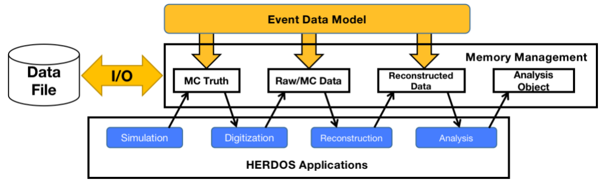
The event data, to be processed by the algorithms is stored in a common storage shared by all Algorithms, named DataStore. Each Algorithm has read and write access to the storage, as shown in the following figure.
The following script shows a simple python script that calls HERDOS to execute a simple data processing task. In this example, an Algorithm named as ��HelloAlg�� is configured. During the event loop, HERDOS will call HelloAlg::execute() for each event. There are a few other modules, such as Sniper and Task. They will be introduced in detail in the developer documentation.
#!/usr/bin/env python
# -*- coding:utf-8 -*-

import Sniper

task = Sniper.Task("task")
task.setLogLevel(2)

import HelloWorld
alg = task.createAlg("HelloAlg")

task.setEvtMax(5)
task.run()
There are a few examples defined under the offline/Example folder, including
offline/Example/AnalysisExample: example of analyzing HERDOS data file
offline/Example/EDMtests: example of reading/writing event data
offline/Example/HelloHist: example of calling
RootWriterto create hitsogramsoffline/Example/HelloTree: example of calling
RootWriterto create TTreesoffline/Example/HelloWorld: example of simple Algorithm, Service and Tool
Run official simulation
There are a few python scripts pre-defined to run detector simulation and reconstruction jobs. After HERDOS is compiled, they are placed under the offline/install/script folder, including:
Full detector simulation:
offline/install/scripts/SimpleSimConfig/devrun.py
Example of running this scripts
External environment
source /cvmfs/herd.ihep.ac.cn/HERDOS/SLC7/Pre-release/ExternalLibs-GCC8.5.0/bashrc.shOffline environment
source /path/to/install/setup.shNow you have all related environment ready run scripts
python offline/install/scripts/SimpleSimConfig/devrun.py  --seed 123 --g4mac comp_vertical-full.g4mac  --particle proton --energy 60 -o ./sim.root -N 3000

  --seed     integer of random number to put into Geant4
  --g4mac    geant4 macro used, examples can be found in /path/to/install/g4macro/*.g4mac, for example comp_vertical-full.g4mac, comp_iso-R1.8m.g4mac, comp_powerlaw.g4mac
  --particle particle type, supported : electron, proton, helium etc, for other nuclei, you can add ion_3_6_3 for Lithum3
  --energy   MC energy in GeV, --energy 0.3 150 if specify an energy range 0.3-150 GeV.
  -o         MC output name.
  -N         number of events used in generation.
Other options: powerlaw you can apply
/gps/ene/type Pow
/gps/ene/alpha -1
/gps/ene/min 0.3
/gps/ene/min 150
All other Geant4 macro parameters are supported in �Cg4mac
MC simulation results
Run official digitalization & reconstruction
In the section of simulation example, we generate 3k MC events of 60GeV proton with vertical direction. Proper digitalization and reconstruction process are required, alike the simulation, these algorithms are treated as packages/modules and can be imported separately.
   python /offline/install/scripts/GlobalTrack/run_recon.py
   usage: run_recon.py --input INPUT --output OUTPUT [--geometry GEOMETRY]
   [--calopca] [--calodigi] [--psddigi] [--fitdigi] [--fitcluster]
   [--fittrack] [--scddigi] [--scdcluster] [--scdtrack] [--globaltrack]
   the following arguments are required: --input, --output
FIT reconstruction example with digitalization, cluster finding and fit track finding
python run_recon.py --input sim.root --output out.root \n
 --fitdigi --fitcluster --fittrack
SCD reconstruction example with digitalization, cluster finding and fit track finding
python run_recon.py --input sim.root --output out.root \n
 --calopca --scddigi --scdcluster --scdtrack
Global track finding with FIT & SCD cluster information \n track reconstruction example with SCD&FIT digitalization, cluster finding and global track finding \n
 python run_recon.py --input sim.root --output out.root \n
 --scddigi --scdcluster --fitdigi --fitcluster --globaltrack
From the scripts, the packages available (not all) in HERDOS are imported here, including digitalizaiton and reconstruction. The order of modules imported are not fixed.
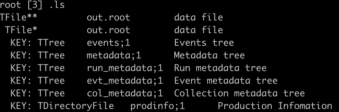
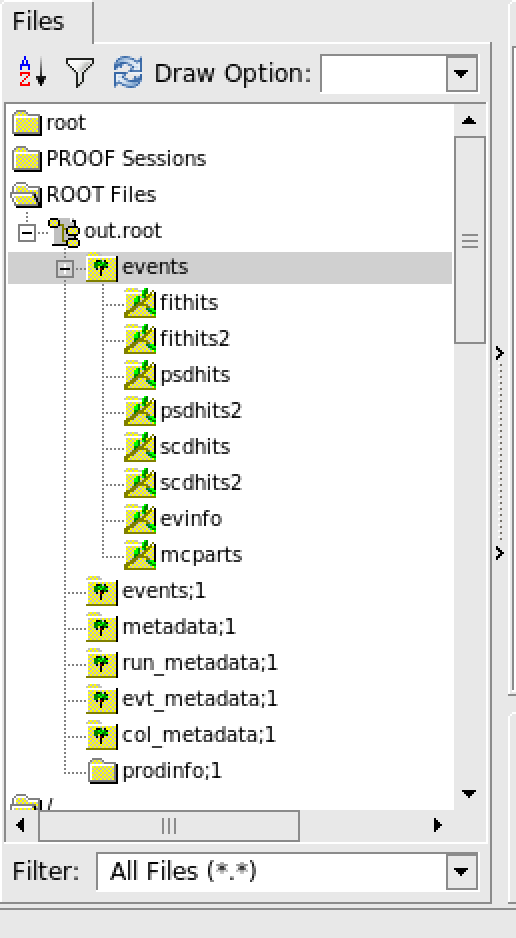
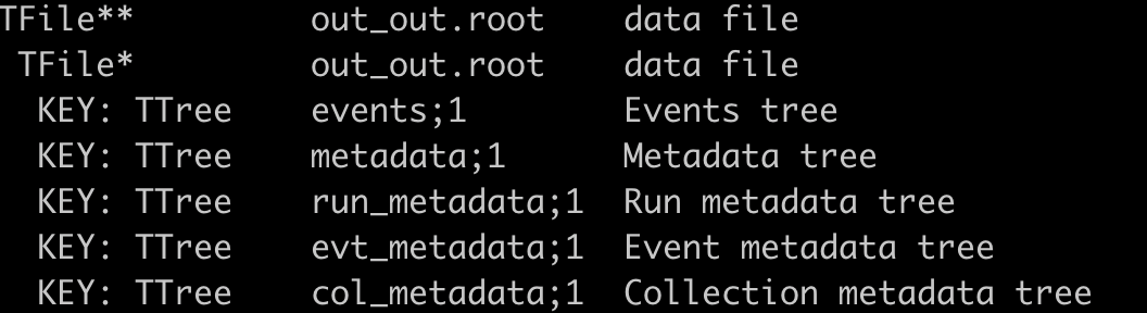
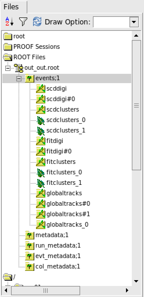
Digitalizatoin & Reconstruction results
The detailed explaination of tree/branch can be found in sector.
Analyse data files
The file format of data files generated by HERDOS is ROOT. The data I/O and event data model is developed based on podio. For complex analysis, where you need to read correlations between EDM objects (e.g. analyze MCParticle together with MC hits), we recommend to write your HERDOS algorithms. A simple example is provided in the AnalysisAlg algorithm under Example/AnalysisExample, as shown below.
bool AnalysisAlg::initialize()
{
    LogInfo << " initialized successfully" << std::endl;
    hist_edep = new TH1D("hist_edep","hist_edep",50,0,0.2);
    return true;
}

bool AnalysisAlg::execute()
{
    LogDebug << "Processing event " << m_iEvt << std::endl;
    ++m_iEvt;

    auto TrackSimHits = getROColl(TrackingSimHitCollection, "scdhits");
    auto CaloSimHits = getROColl(CaloSimCellCollection, "calohits");

    if (TrackSimHits) {
        // Do some analysis here.
    }

    if (CaloSimHits) {
        for (size_t i=0; i<CaloSimHits->size(); ++i) {
            auto edep = CaloSimHits->at(i).getEdep();
            hist_edep->Fill(edep);
        }
    }
    return true;
}
The code example above reads the simulated SCD and calorimeter hits from the detector simulation output file, using C++ macro getROColl, then loop through the collection of hits and draw some histograms. Full code and python script can be found in offline/Examples/AnalysisExample/src/AnalysisAlg.cc, offline/Examples/AnalysisExample/src/AnalysisAlg.cc and offline/Examples/AnalysisExample/scripts/AnalysisAlg.py.
Detailed introduction of EDM classes and the data management services will be introduced in the developer documentation.
If you would only like to perform quick and simple analyze, writing ROOT macro scripts is also possible. But you need also setup the HERDOS runtime environment before running the analysis, since ROOT needs to load dictionaries of EDM classes. A simple ROOT script is provided as an example:
#include "TFile.h"
#include "TChain.h"
#include <vector>

using namespace edm;
void ReadEDM(){
  TChain *data = new TChain("events");
  data->AddFile("data_1.root");
  data->AddFile("data_2.root");

  vector<CaloSimCellData>* calohits=0;
  data->SetBranchAddress("calohits",&calohits);

  TCanvas* c = new TCanvas("c","c",800,600);
  c->SetGrid();

  TH1D* h1 = new TH1D("h1","energy deposit",50,0,0.2);

  int nEntries=data->GetEntries();
  for(int i=0;i<nEntries;i++){
    data->GetEntry(i);
    std::cout << "size: " << calohits->size() << std::endl;
    for(size_t j=0;j<calohits->size();j++){
      h1->Fill(calohits->at(j).edep);
    }
  }

  h1->Draw();
}
The above script opens ROOT files, and read the EDM objects directly from TTrees. Podio uses the format of std::vector of EDM objects to for persistent data storage. The concreate EDM classes are defined in the offline/EventDataModel/DataModel/data_layout.yml file, while the c++ code is automatically generated. Please reach to the Doxygen documentation, or check code directly under offline/EventDataModel/DataModel.
Profile your code using jMonitor
Sometimes it is nesessary to profile the performance of your application software, such as measuring the CPU usage, memory usage or disk I/O activities as a function of time. In HERDOS we provide the jMonitor command to profile software performance. The basic usage is listed below.
usage: jMonitor [-h] [-T MAXTIME] [-M MAXVIR] [--enable-parser] [-p FATALPATTERN] [--enable-monitor] [--enable-perf] [--enable-io-profile]
                [-i INTERVAL] [-l {root,matplotlib}] [-b {ps,prmon}] [--enable-plotref] [-f PLOTREFFILE] [-o PLOTREFOUTPUT] [-m {Kolmogorov,Chi2}]
                [-c HISTTESTCUT] [--gen-log] [-n NAME]
                command [command ...]

positional arguments:
  command               job to be monitored

optional arguments:
  -h, --help            show this help message and exit
  -T MAXTIME, --time-limit MAXTIME
                        Time limit of process (s), if exceeded, process will be killed
  -M MAXVIR, --memory-limit MAXVIR
                        Memory limit of process (Mb), if exceeded, process will be killed
  --enable-parser       If enabled, log of the process will be parsed
  -p FATALPATTERN, --pattern FATALPATTERN
                        Python re patterns for the parser
  --enable-monitor      If enabled, process will be monitored (memory, cpu)
  --enable-perf         If enabled, process will profiled via perf
  --enable-io-profile   If enabled, process disk IO will profiled
  -i INTERVAL, --interval INTERVAL
                        Time interval for monitor
  -l {root,matplotlib}, --plotting-backend {root,matplotlib}
                        Backend for plotting monitoring figures
  -b {ps,prmon}, --monitor-backend {ps,prmon}
                        Backend performance profiling
  --enable-plotref      If enabled, results of the process will be compared
  -f PLOTREFFILE, --plotref-files PLOTREFFILE
                        reference file for plot testing
  -o PLOTREFOUTPUT, --plotref-output PLOTREFOUTPUT
                        output root file for plot comparison
  -m {Kolmogorov,Chi2}, --histtest-method {Kolmogorov,Chi2}
                        Method of histogram testing
  -c HISTTESTCUT, --histtest-cut HISTTESTCUT
                        P-Value cut for histogram testing
  --gen-log             whether to generate log file
  -n NAME, --name NAME  name of the job